Ref. Open: UKF

레이블이 UKF인 게시물을 표시합니다. 모든 게시물 표시

2014년 10월 1일 수요일

github에서 Rsimulator 보기

Rsimulator 소개

Rsimulator는 Visual studio 2010, C++, opencv 기반으로 만들어진 이동 로봇 시뮬레이터입니다.

라이센스

Rsimulator는 GPL을 따릅니다.(GPL 한글 번역 전문)

기업, 학교, 개인이 마음대로 개작하고 재배포해도 좋지만, 개작된 소프트웨어의 소스코드는 GPL에 따라 공개되어야 하고 Rsimluator를 사용했다는 것을 밝혀야 합니다.. Rsimulator를 공공의 목적으로 공개하는 이유이기도 합니다.

기능 명세

로봇 설정(두 개의 바퀴와 하나의 캐스터)
장애물 환경 디자인(사각형, 원형, 직선 등)
초음파, 레이저 센서 스캔 시뮬레이션
점유 격자 지도 작성 시뮬레이션
전역 경로 계획 시뮬레이션
지역 경로 계획 시뮬레이션
UKF SLAM 시뮬레이션

소스 다운로드 방법

git에 대해 익숙하신 분은 본 글 상단의 링크를 참고하시면 됩니다.

처음이신 분은 본 글 상단의 링크를 통해 Rsimulator git을 fork하고

github for windows를 통해 clone을 받으시면 됩니다.

간단 사용 방법

처음 화면에 몇 개의 원이 뿌려져 있습니다. 랜덤하게 생성된 35의 점(랜드마크 입니다.) r 키로 적당한 크기의 로봇의 생성시키고 space bar를 누르면 정해진 궤적을 따라가면서 SLAM을 수행합니다.

왼쪽 메뉴의 DT, VFF, VFH를 선택하면 로봇이 다르게 반응합니다. 자세한 설명서는 시간이 허락하면 작성할 계획입니다.

시뮬레이터 개선 계획

현재는 없습니다. 다만, 본 프로그램을 사용하시는 분이 좋은 아이디어를 바탕으로 개선한 내용을 github에 pull하고 싶으시다면 적극 환영합니다. 공동으로 작업하고 싶은 의향도 있습니다. 그것이 공중 소프트웨어의 본질이라고 생각합니다.

시뮬레이터 실행 화면

2014년 9월 24일 수요일

EKF vs. UKF 비선형 상태 변환 성능 비교

필터에서 상태 천이 함수가 선형인 경우엔 Kalman filter를 사용합니다. 상태 천이 함수가 비선형인 경우에는 EKF, UKF, PF를 사용하게 되는데, 이 때 간단한 비선형 천이 함수를 이용하여 EKF와 UKF의 성능이 어떤 차이가 발생하는지를 확인해보고자 합니다.

다음에 제시한 예제는 $x, y$ domain에서 $ \rho, \theta $로 변환하는 기본적인 비선형 천이 함수를 이용해 EKF와 UKF가 예측한 $2\sigma$를 표현한 타원을 보면 직관적으로 그 차이를 이해할 수 있습니다.

http://refopen.blogspot.com/2014/09/ekf-vs-ukf.html

Magnus Nørgaard는 derivative-free filter인 UKF가 taylor series의 2차까지 근사화하므로 비선형 함수에서 더욱 정확한 성능을 보장한다고 주장했습니다.

http://www.sciencedirect.com/science/article/pii/S0005109800000893

EKF vs. UKF 비선형 상태 변환 성능 비교 예제

filterComparison

% EKF vs. UKF
% 2014. 9. 24
% refopen.blogspot.com
% This example intuitively shows that the difference between EKF and UKF
% when state transition is non-linear function.

function filterComparison()

Create real data

Create some real data points(1000points)
$\sigma_x = 5, \sigma_y = 3$

sigmax = 5;
sigmay = 3;
rx = randn(1000, 1)*sigmax;
ry = randn(1000, 1)*sigmay;

% real data points and MLE parameter estimation
figure(001);
plot(rx, ry, 'r.');
xlabel('x');
ylabel('y');
axis([-15 15 -15 15]);
[x, P] = MLEnPlot(rx, ry);

$r = \sqrt{x^2+y^2}$
$\theta = tan^{-1}\frac{y}{x}$

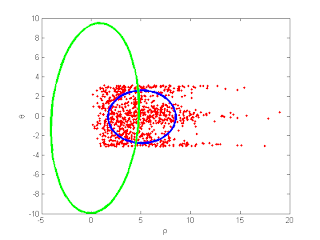
figure(002);
rho = sqrt(rx.^2 + ry.^2);
theta = atan2(ry, rx);
plot(rho, theta, 'r.');
xlabel('\rho');
ylabel('\theta');
MLEnPlot(rho, theta);
fprintf('press any key to continue...\n');
pause;

press any key to continue...

Extended Kalman Filter

Find out jacobian matrix when it transformed by non-linear state transition matrix.
$J = \left[\begin{array}{cc} \frac{\partial r}{\partial x} & \frac{\partial r} {\partial y} \\ \frac{\partial \theta}{\partial x} & \frac{\partial \theta}{\partial y} \end{array}\right]$
Now, prediction of covariance matrix at the pridiction step $P_{r\theta}=JP_{xy}J^T$

q = x(1).^2 + x(2).^2;
J = [x(1)/sqrt(q) x(2)/sqrt(q); -x(2)/q x(1)/q];

xekf = [sqrt(x(1).^2 + x(2).^2) atan2(x(2), x(1))];
Pekf = J*P*J';

% draw ellipse
e = make_covariance_ellipses(xekf, Pekf);
hold on; plot(e(1, :), e(2, :), 'g-' , 'LineWidth', 3); hold off;
fprintf('press any key to continue...\n');
pause;

press any key to continue...

Unscented Kalman Filter

Set up some values

D = length(x);  % dimension
N = D*2 + 1;

samples are should be generated.

scale = 3;
kappa = scale-D;

% Create unscented sample points
Ps = chol(P)' * sqrt(scale);
ss = [x', repvec(x',D)+Ps, repvec(x',D)-Ps];

$(x, y) \rightarrow (\rho, \theta)$

rho = sqrt(ss(1, :).^2 + ss(2, :).^2);
theta = atan2(ss(2, :), ss(1, :));
x = [rho; theta];

idx = 2:N;
xukf = (2*kappa*x(:,1) + sum(x(:,idx),2)) / (2*scale);
diff = x - repvec(xukf,N);  % weighted sample cov.
Pukf  = (2*kappa*diff(:,1)*diff(:,1)' + diff(:,idx)*diff(:,idx)') / (2*scale);

% draw ellipse
e = make_covariance_ellipses(xukf, Pukf);
hold on; plot(e(1, :), e(2, :), 'k-' , 'LineWidth', 3); hold off;

end

function [x, P] = MLEnPlot(x, y)
phatx = mle(x);
phaty = mle(y);
x = [phatx(1) phaty(1)];
P = [phatx(2) 0; 0 phaty(2)];
e = make_covariance_ellipses(x, P);
hold on; plot(e(1, :), e(2, :), 'b-' , 'LineWidth', 3); hold off;
end

from timbailey's matlab utility

function p= make_covariance_ellipses(x,P)
% compute ellipses for plotting state covariances
N= 60;
inc= 2*pi/N;
phi= 0:inc:2*pi;

lenx= length(x);
lenf= (lenx-3)/2;
p= zeros (2,(lenf+1)*(N+2));

ii=1:N+2;
p(:,ii)= make_ellipse(x(1:2), P(1:2,1:2), 2, phi);

ctr= N+3;
for i=1:lenf
    ii= ctr:(ctr+N+1);
    jj= 2+2*i; jj= jj:jj+1;

    p(:,ii)= make_ellipse(x(jj), P(jj,jj), 2, phi);
    ctr= ctr+N+2;
end
end
%
%

function p= make_ellipse(x,P,s, phi)
% make a single 2-D ellipse of s-sigmas over phi angle intervals
r= sqrtm(P);
a= s*r*[cos(phi); sin(phi)];
p(2,:)= [a(2,:)+x(2) NaN];
p(1,:)= [a(1,:)+x(1) NaN];
end

function x = repvec(x,N)
x = x(:, ones(1,N));
end